Retinal image computation software
/*************************************************************************************
These programs are free software; you can redistribute
them and/or modify
them under the terms of the GNU General Public License as
published by
the Free Software Foundation; either version 2 of the License, or
(at your option) any later version.
*************************************************************************************/
- The screen's Spectral Power distribution (SPD).
- The Judd51
 ,
,  ,
,  .
.
- The Judd Specs matrix.
- The Zernike coefficients modelling the
wave aberration.
- Cones fundamentals.
- The screen's Spectral Power
distribution (SPD).
The CRT
calibration using a spectroradiometer provides the three
gun's Spectral Power Distribution (SPD).
This SPD is
used to decompose the displayed image into wavelengths (See Formulas).
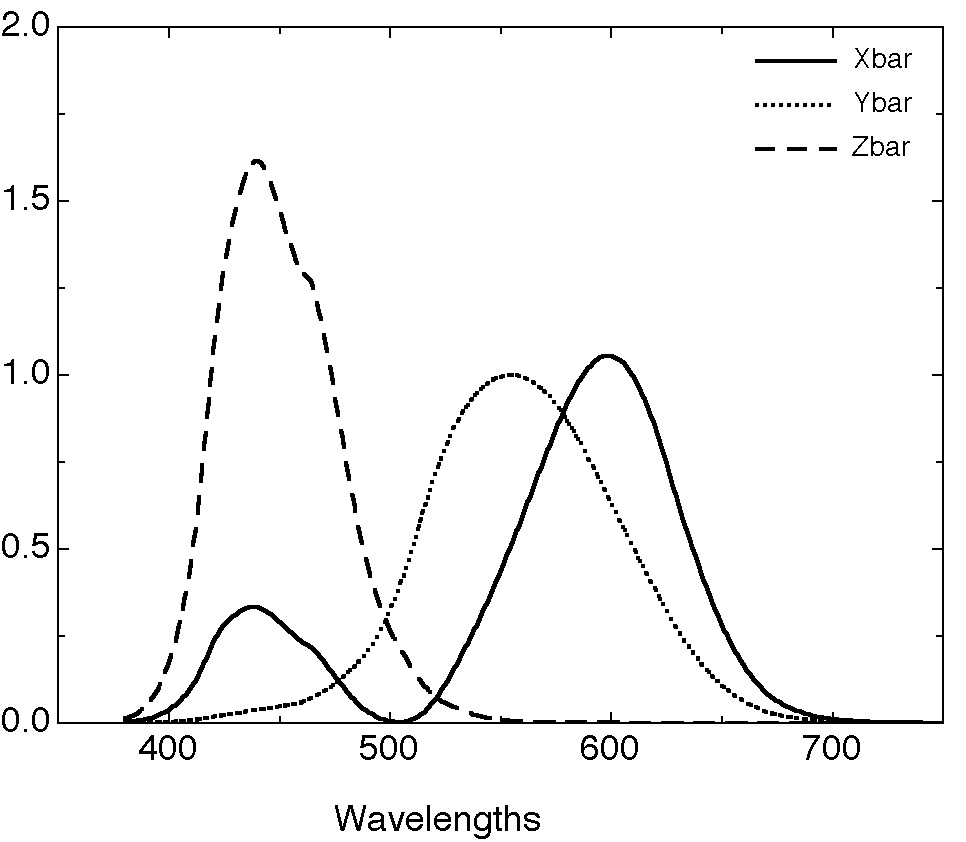
The , , color matching functions are represented in the
figure below.
The Judd Specs matrix gives the
tristimulus values for the three guns.
Note that the luminances (YR,
YG, YB) are normalised so the Green luminance (YG)
is set to 100.0.
We give below an example of Judd
Specs file corresponding to one of the Shevell's lab monitors.
|
x
|
y
|
Y
|
Red
|
0.6266
|
0.3442
|
26.4531
|
Green
|
0.2908
|
0.6145
|
100.0
|
Blue
|
0.1522
|
0.0831
|
15.6325
|
See the Formula's page for information about
the Judd specs computation.
- The Zernike coefficients
modelling the wave aberration.
Here is an example
set of typical Zernike coefficients (Thibos et al. 2002).
Zernike mode number
|
Coefficient value
|
1
|
-0.7380
|
2
|
0.5802
|
3
|
0.6098
|
4
|
0.1641
|
5
|
0.8314
|
6
|
0.1405
|
7
|
-0.2377
|
8
|
0.1395
|
9
|
0.1944
|
10
|
0.1191
|
11
|
0.0287
|
12
|
0.0002
|
13
|
0.1293
|
14
|
-0.0081
|
15
|
-0.0068
|
The
software can either load the Cones fundamentals or compute them from
Judd51 , ,
 Conversion matrixfrom Judd'51
colormatching functions:
Conversion matrixfrom Judd'51
colormatching functions:
![$ \left[
\begin{tabular}{ c}
L \\
M\\
S \\
\end{tabular}\right]$](Manual/RetImg/img7.png) =
![$ \left[
\begin{tabular}{ c c c }
0.15514 & 0.54312 & -0.03286\\
-0.15514 & 0.4...
... c}
$\overline{x}$\\
$\overline{y}$\\
$\overline{z}$\\
\end{tabular}\right]
$](Manual/RetImg/img8.png)
|
/***************************************************************************
-------------------
Last modification : march 10th 2005
Florent Autrusseau
email : Florent.Autrusseau@univ-nantes.fr
-------------------
***************************************************************************/